Confounding: why two groups can differ for other reasons

01The pump and the brewery

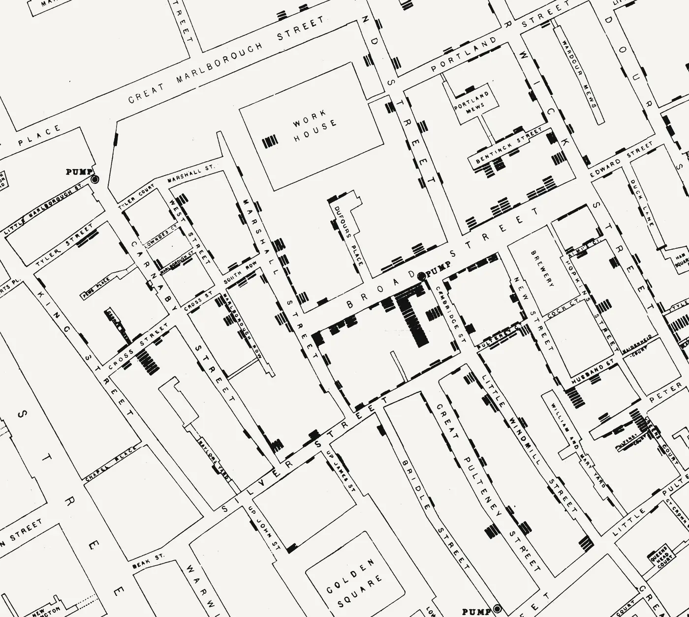
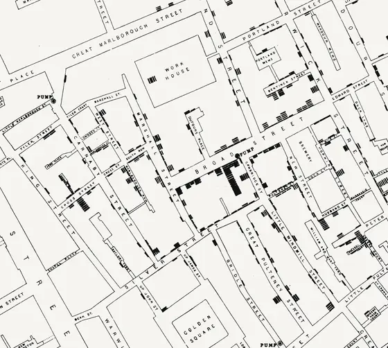
In the 1854 Soho outbreak, John Snow mapped cholera deaths and noticed a cluster near the Broad Street pump. A map alone was not enough. Neighbors share many features, including air, drains, occupations, habits and often a water supply.

Snow's investigation checked who drank from the pump and who did not. He reported that a nearby brewery had no severe cholera among its workforce, and the proprietor said the workers did not use the street pump and had other supplies. Residents farther away who drank water brought from Broad Street were affected, so distance alone was not the same as exposure.

The comparison that mattered followed the water rather than the circle. People without the suspected exposure nearby and people with it at a distance separated the water explanation from simple proximity.

02What a confounder is

A confounder is a variable associated with both the suspected cause and the outcome. It can create an apparent relationship that is not causal, or hide a real one. Living near a pump is associated with many other things, including crowding, sanitation and occupation.

Confounding is often invisible in the outcome data itself. Two groups can differ in mortality for reasons unrelated to the exposure under study, and the difference can look like evidence for that exposure.

Interpretation: good comparisons begin with a list of plausible confounders, then ask how each would be controlled, measured or tested. Where control is impossible, the limits of the conclusion should be stated plainly.

Two common mistakes follow from this. The first is to adjust for everything measurable without asking whether some measured variable is itself a result of the exposure, which can distort the comparison. The second is to assume that the confounder list is complete. A list reflects what the investigators thought to measure, and unmeasured factors remain possible.

03Natural experiments

Sometimes a comparison arises without the researcher choosing the groups. A water source changes, a policy starts in one district but not another, or a supply is interrupted. Such events can approximate an experiment, because the assignment of exposure is driven by circumstances unrelated to the outcome.

Snow's removal of the pump handle in September 1854 was an intervention, not a controlled experiment. The outbreak was already declining before the handle was removed, so timing alone cannot measure the intervention's effect. A natural experiment needs a comparison that holds the other factors as constant as possible.

For any natural experiment, the question is whether the groups differ mainly in the exposure. If they also differ in income, age or timing, the comparison needs adjustment or should be treated as suggestive.

04The 1918 influenza cities

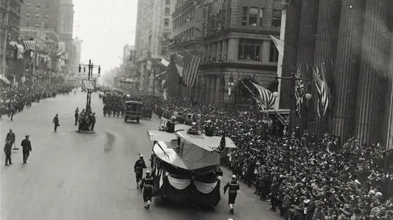
In 1918, U.S. cities adopted public-health measures at different times and with different intensity, and the influenza pandemic produced different wave patterns from one city to another. Bootsma and Ferguson asked whether differences in measures could explain the variation in mortality among cities.

Their abstract reports that city-specific excess mortality in 1918 correlated with 1917 mortality, which suggests some intrinsic variation in overall mortality, possibly linked to sociodemographic factors. Among 23 cities with partial intervention data, earlier introduction of interventions correlated even more strongly with excess mortality. An epidemic model fitted to weekly data for 16 cities reproduced the observed patterns and was used to estimate the impact of interventions.

The 1917 correlation is a confounding warning. A city that was already more vulnerable might also have adopted measures at a different time, so the effect of the measures has to be separated from baseline differences. The model is designed to address that concern, but its estimates still rest on assumptions.

05Season as a confounder

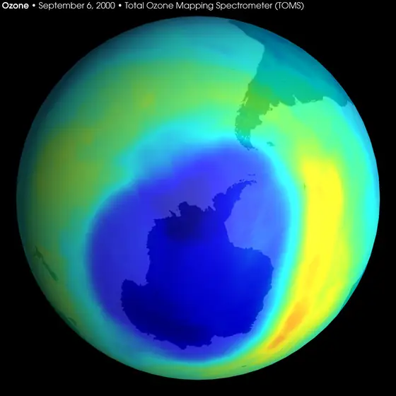
Time can confound a comparison. Antarctic ozone varies strongly with the seasons, so comparing a spring reading in one year with a summer reading in another would mix a natural cycle with a long-term change.

The case summary emphasizes that the decisive comparison was between spring values in different years, not between arbitrary seasons. Farman and colleagues' 1985 Nature paper, whose title refers to losses of total ozone in Antarctica and to seasonal chemistry, is the primary report of the spring decline that the case describes.

Seasonal confounders are easy to overlook when a series looks like a single trend. The safe habit is to compare equivalent periods before drawing a conclusion about change.

The same logic applies when the seasonal cycle is strong and the record is short. A few years of data may show a shift in one season, but the investigator still has to check that the pattern is not an artifact of the particular years chosen.

06Designing a fairer comparison

Start with the outcome and list the factors that differ between the groups. For each one, decide whether to match, stratify or adjust for it, or look for a case where it varies independently of the exposure.

Check the timing. A decline that began before the intervention can make the intervention look more effective than it was. Compare trends before and after, and look for exceptions that the proposed explanation must also accommodate.

Record the exposure data carefully. Many comparisons weaken because the record of exposure is incomplete. The 1918 city analysis worked with partial intervention data for some cities, and its authors had to account for that in the analysis.

Pre-specify the comparison where possible. Deciding in advance which groups, periods and outcomes will be compared limits the temptation to choose whichever comparison looks best after the data arrive.

07What a comparison can and cannot show

A well-designed comparison can rule out some alternatives and make others less likely. It rarely proves a single cause, especially in observational studies where exposure was not randomized.

Snow's investigation and the 1918 city study both show that an intervention can be effective while the evidence remains imperfect. Their strength lies in testing each explanation against the cases it does not predict well.

The open question in any comparison is which unmeasured factor might still explain the difference. Naming that factor honestly is part of the method.

Comparisons are most persuasive when they could fail. A good comparison states in advance what pattern would undermine the proposed explanation, and then reports whether that pattern appeared.